Oh My, Oh Miocene!

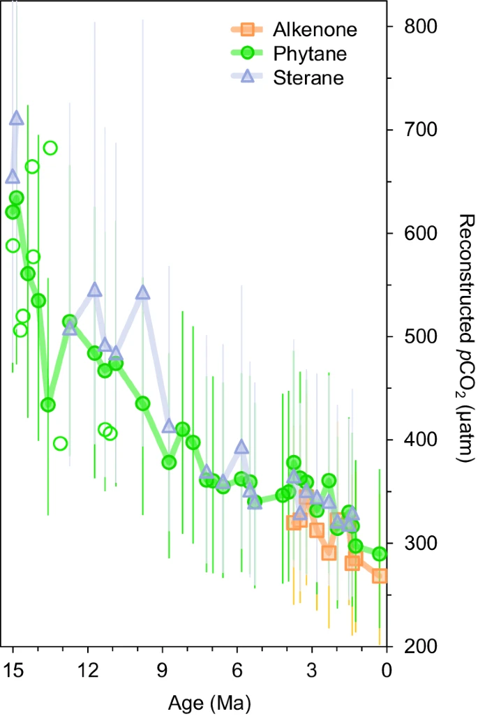
A recent paper suggested that ‘climate sensitivity’ derived from a new paleo-CO₂ record is around 7.2ºC (for equilibrium climate sensitivity ECS) and ~13.9ºC (Earth System Sensitivity – ESS) for a doubling of CO₂. Some press has suggested that this means that “Earth’s Temperature Could Increase by 25 Degrees” (F). Huge if true! Fortunately these numbers should not be taken at face value, but we need to dig into the subtleties to see why.

The paper in question is Witkowski et al. (2024), which was published in Nature Communications. The meat of the paper is a reconstruction of paleo-CO₂ from relatively new proxies – sterane and phytane δ¹³C ratios – derived from phytoplankton living in the ocean photic zone in the coastal ocean off of California.

The geochemistry here is quite involved, and I’m not qualified to assess how well this has been done, but it’s sufficient to take this as perfectly valid for the points I’ll make here. There are often somewhat heroic assumptions made in deriving paleo atmospheric CO₂ from molecular markers, but the overall results (see left hand figure) – that CO₂ went from 650 ppm 15 Million years ago (Ma) to 280 ppm in the most recent data point (close to the long term pre-industrial average), is not dramatically different from other recent compilations (such as CenCO2PIP (2023)) (right hand figure). The novelty here is (I think) that this change is calculated in a single core over the whole 15 Ma interval (albeit at a roughly 500,000 yr sampling interval).

The peak value roughly 15 Ma ago, corresponds the climate period sometimes referred to as the Miocene Climate Optimum (MCO), possibly the warmest period in the last 20 million years, with very little remaining glacial ice, and roughly 8ºC above the pre-industrial in the global mean surface temperature (Ring et al, 2022).

Astute readers will perhaps have already have done a quick back of the envelope calculation, given that the radiative forcing from 280 ppm to 650 ppm is around 4.7 W/m² (using the Etminan et al. (2016) formula and assuming an average N₂O value of 272 ppb – roughly 25% larger than the value for 2xCO2, 3.8 W/m²), to get a naive ‘Earth System Sensitivity’ of 8/4.7*3.8 = 6.5ºC for a doubling of CO₂. This is quite a bit less than the Witkowski et al conclusion. So what is going on?

Sensitivity, Schmensitivity

First off, we need to be crystal clear about what our definition of climate sensitivity is: It is the change of global mean temperatures expected after a doubling of CO₂. However, we frequently assume that some things remain constant. For instance, the standard ‘Charney Sensitivity’ or Equilibrium Climate Sensitivity (ECS) assumes that ice sheets don’t change. The broader concept of Earth System Sensitivity (ESS) allows for responses in the ice sheets, vegetation etc. Responses in atmospheric composition (dust, ozone, aerosols etc.) are sometimes included (or not!). Indeed, one can define a whole series of climate sensitivities depending on what feedbacks are included and over what time-scale:

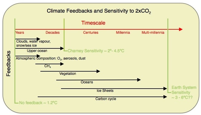
So what are we dealing with here? Clearly, over the last 15 Ma, there have been big changes in the ice sheets, sea level (and presumably vegetation, and atmospheric composition), and some changes in solar irradiance as well as variations in continental configurations, so we should factor these things in to get to an ECS that is commensurate with what we talk about in the modern period. The authors make some attempt to do that by assuming a forcing of roughly 2 W/m² (=66 m * 0.0308 W/m³) associated with change of ice sheets from PI to MCO. That would reduce the implied sensitivity to CO₂, to 8/(4.7+2)*3.8 = 4.5ºC. However, they don’t calculate the influence of the other factors – such as the Rocky mountain range and the Andes in the Americas being lower elevation, changing circulation patterns and temperatures independent of CO₂ (paleogeography effects), and the solar irradiance changes.

In work that we did a while ago on the Pliocene (3 Ma) Lunt et al, 2012, we calculated the paleogeography effect was worth 0.7ºC, and one might expect it to be greater for the earlier Miocene period (maybe 1ºC?). The solar irradiance has increased about 4.4% over the Phanerozoic (540 Ma), and so over 15Ma, that’s about 1.6 W/m² in TSI, and thus about 1.6*0.7/4 = 0.3 W/m² in solar forcing. Combining these effects with the prior calculation, you get (8-1)/(4.7+2-0.3)*3.8 = 4.2ºC – well within the scope of other ECS estimates. Note that here we are implicitly assuming that any vegetation or composition changes (including CH₄, N₂O, ozone and aerosols) are only changing because of changes in temperature and are thus feedbacks, not independent forcings – that’s different from how these are treated in historically-based estimates (where they have changed directly due to human activities). We could instead try to scale the N₂O and CH₄ changes (including indirect effects) based on glacial to interglacial transitions, and that would imply an ~25% increase in the forcing. So then we’d end up with (8-1)/(4.7*1.25+2-0.3)*3.8 = 3.5ºC for a sensitivity not including those feedbacks. Again, not too different from what one would expect.

Similarly, we could estimate the ESS (by not including the ice sheet term, and assuming that all composition change was a feedback too) as 7/(4.7-0.3)*3.8=6.0ºC, again, not so far off existing estimates. Of course, there are significant uncertainties in all of this that need to be taken into account, so the constraints are not as tight as one might like (and I haven’t mentioned the possibility that ESS/ECS might be varying as a function of the base state…).

But…

I’ve shown that neither the existing temperature reconstructions nor the new CO₂ reconstructions for the Miocene obviously suggest some massive climate sensitivity, so where do the Witkowski authors get their numbers from? They do two things that are somewhat non-standard. First, they separate out different latitudinal bands (SH and NH mid-latitudes, tropics, and the NH high latitudes – and from Table 1, it’s clear that they assume the (unsampled) SH high latitudes are changing the same as the NH high latitudes). This isn’t such an obvious assumption. Second, they calculate the sensitivities by regressing the regional temperature reconstructions with radiative forcing calculated from the CO₂ changes, and then estimate the global sensitivity using a weighted mean of the regional regressions.

The authors used a (slightly non-standard) linear regression method between CO₂ forcing and T that takes into account varying uncertainties in both the sets of values (unlike ordinary least squares). The specific algorithm they use is ‘fitexy‘ which comes from Numerical Recipes (1992). It was not immediately obvious (to me, a non-statistician) what this is based on, but I think it’s related to a special case of what is now called York regression (with uncorrelated uncertainties). There are two consequences of this choice; first, it’s important to have reasonable estimates for the uncertainties (which can be hard), and second, it’s not linear i.e. the regression for the global mean, doesn’t equal the global mean of the regional regressions (I’ll demonstrate that below). Finally, and this will be important, the uncertainties on the regression can be quite large.

Adventures in replication

We’ve often discussed the ease and utility of replication, and this paper is a good example of why it’s important. In order to to see why the chosen procedure gives the numbers it does, we need to work through the calculations, and perhaps test some of the assumptions. Unfortunately, the sensitivity calculations were not part of the supplementary material (IMO they should have been) but two coauthors of the paper were helpful and sent me a spreadsheet of these results and clarified a few details.

The first thing to look at is the radiative forcing for the CO₂. The authors used the formula (their Eqn. 3), which is taken from Etminan et al. (2016). [Note that the equation as published in this paper has two typos in the coefficients: a₁ and c₁ should be negative not positive]. Secondly, there is a small dependency in this formula on the average N₂O concentration over the period, which is unknown, and the authors don’t mention what they used. Through a bit of trial and error, I found that I could match their calculation assuming N₀=272 ppb and C₀ = 278 ppm (reasonable pre-industrial levels), so the radiative forcing for 2xCO2 is 3.8 W/m², and the forcing at 650 ppm is 4.7 W/m². The uncertainties in the CO₂ are given as almost constant % differences for the one sigma lower (33%) and upper bounds (28.5%) and are thus quite large.

Temperatures

The temperatures being used are from Herbert et al (2016) who produced stacked estimates of changes from the Miocene to present for the different regions mentioned above (all available in their supplementary material). These temperatures don’t appear to be inconsistent with the global estimates mentioned above, but are usefully segregated by broad latitude bands, and come with an uncertainty based on the standard deviation of the estimates of the temperatures that go into each stacked average. I found a couple of errors in this spreadsheet, but was able to interpolate these stacked values and their uncertainty to get something close to what the Witkowski et al authors used. Note that the tropical data is perhaps not accurate before ~8 Ma, so the authors only use the tropical regression over 0-8Ma, while the other regions use most of the last 15 Ma.

Drum roll please…

With just a few lines of R script I was then able to use the york function using the given CO₂ and it’s uncertainties, and the temperatures and their standard deviation as given by Herbert et al. I’m not sure this is correct – surely it should be the standard error on the stacked temperatures that should be used? but this turns out to be basically irrelevant because the dominant uncertainty is in the CO₂. [Replicating this also revealed that in Figure 3 two lines are mislabeled (the NH mid-latitudes is actually green, and the SH mid latitudes is cyan), and that Figure S5 (panel c) is plotting the wrong regression.]

For the first calculation, simply correlating the regional temperatures to CO₂ and then area-averaging the regressions to calculate a naive global ‘ESS’, I get similar values to Witkowski et al., roughly 3.8 K/(W/m²), which once you convert by multiplying by 3.8 W/m², is roughly 14.6ºC for a doubling of CO₂ (Note Witkowski et al use 3.7W/m², which is inconsistent with what they use for the forcing in the regression). However, the uncertainty on this number is huge: ±15.3ºC (95% CI)!! Using the land-ice correction as the authors did, I get the ‘ECS’ as 7.2±3.1ºC (95% CI) – again a very high (though proportionately slightly smaller) uncertainty. Basically the fits for the regressions are not very good, though it’s a little better for the land-ice-corrected calculation.

I mentioned above that York regression is not a linear operator: if I take the global mean of the regional regressions, it does not equal the regression of the global mean. I can show this doing the regressions on just the 0-8Ma segments where I can calculate a global mean temperature (and with suitably weighted uncertainties) and compare that to a global mean of the regional regressions. Note that in all of these estimates there is an assumption that the SH high latitudes are changing just like the NH high latitudes. I get that for the global ECS regression, a sensitivity of 7.1±4.2 ºC, while for the global mean of the regional regressions, I get 6.6±7.0 ºC – similar, but not the same. Both these estimates use the same raw data and it’s uncertainties, and so this raises questions about what the right method to use is if the goal is constrain the global mean sensitivity.

Nonetheless, the global temperatures allow us to see quite easily why the uncertainties in the regression coefficients are so large. As in the paper, I plot the global mean temperatures (including their one-sigma standard deviation) against the estimated CO₂ level and its uncertainty. As in the paper too, I don’t use the data earlier than 8Ma (black open circles) because of the reported problems with the tropical temperature proxy. I plot both the York regression and what you’d get with OLS for reference.

<img decoding="async" width="600" height="563" src="https://www.realclimate.org/images//witkowski_ess-600×563.png" alt="Global temperature estimates from Herbert et al, plotted against radiative forcing from Witkowski (with ± 1 sigma). Only data (in red) are used in the regression (

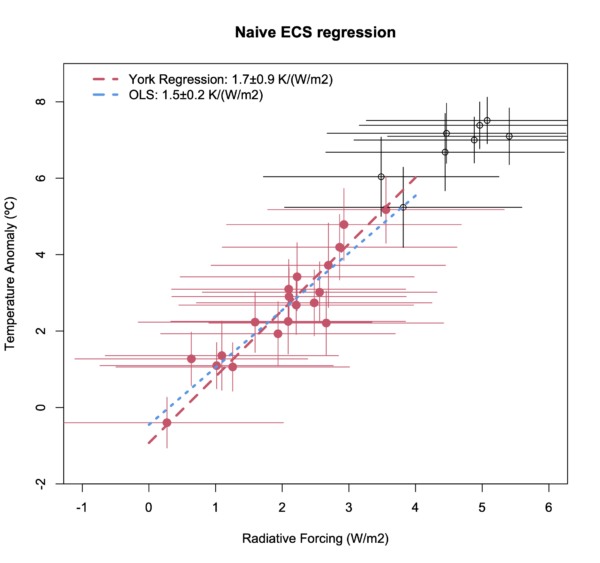
In both cases the errors in the CO₂ estimates dominate the uncertainty (making the issue of what sigma to use for the temperatures moot). Indeed, the errors are so broad that the results don’t even preclude a negative ESS!

As I mentioned above, more sophisticated estimates of both the ESS and ECS could be made using corrections for paleogeography change and the solar irradiance increase, and that would likely reduce the values, but the bottom line from this replication is that the uncertainties in this methodology with this data, are just too large to be useful constraints.

Interestingly, the peer review for the paper is online here, and (perhaps unsurprisingly) the reviewers didn’t discuss whether these calculations would be easily replicable nor what the uncertainties in the sensitivity were. Given the dramatic results, I think this was a bit of an oversight.

What it means

Papers like this – which have good new primary data and somewhat overconfident implications – are relatively common. Digging into why seemingly dramatic results are so overconfident often needs a deep dive into the calculations, and this should be something that could be checked in peer review. However, this is probably too much to ask reviewers to check as a matter of course (since it takes far more time and could just further decrease the acceptance rate for review requests), but maybe editors could commission special replicators to check this stuff specifically (and maybe even pay them for the service!).

Bottom line: this paper usefully adds to the database for paleo-CO2 value, but on its own does not further constrain actual global ESS and ECS estimates, breathless headlines notwithstanding!

References

1. 
   C.R. Witkowski, A.S. von der Heydt, P.J. Valdes, M.T.J. van der Meer, S. Schouten, and J.S. Sinninghe Damsté, “Continuous sterane and phytane δ13C record reveals a substantial pCO2 decline since the mid-Miocene”, Nature Communications, vol. 15, 2024. http://dx.doi.org/10.1038/s41467-024-47676-9

2. 
   . , B. Hönisch, D.L. Royer, D.O. Breecker, P.J. Polissar, G.J. Bowen, M.J. Henehan, Y. Cui, M. Steinthorsdottir, J.C. McElwain, M.J. Kohn, A. Pearson, S.R. Phelps, K.T. Uno, A. Ridgwell, E. Anagnostou, J. Austermann, M.P.S. Badger, R.S. Barclay, P.K. Bijl, T.B. Chalk, C.R. Scotese, E. de la Vega, R.M. DeConto, K.A. Dyez, V. Ferrini, P.J. Franks, C.F. Giulivi, M. Gutjahr, D.T. Harper, L.L. Haynes, M. Huber, K.E. Snell, B.A. Keisling, W. Konrad, T.K. Lowenstein, A. Malinverno, M. Guillermic, L.M. Mejía, J.N. Milligan, J.J. Morton, L. Nordt, R. Whiteford, A. Roth-Nebelsick, J.K.C. Rugenstein, M.F. Schaller, N.D. Sheldon, S. Sosdian, E.B. Wilkes, C.R. Witkowski, Y.G. Zhang, L. Anderson, D.J. Beerling, C. Bolton, T.E. Cerling, J.M. Cotton, J. Da, D.D. Ekart, G.L. Foster, D.R. Greenwood, E.G. Hyland, E.A. Jagniecki, J.P. Jasper, J.B. Kowalczyk, L. Kunzmann, W.M. Kürschner, C.E. Lawrence, C.H. Lear, M.A. Martínez-Botí, D.P. Maxbauer, P. Montagna, B.D.A. Naafs, J.W.B. Rae, M. Raitzsch, G.J. Retallack, S.J. Ring, O. Seki, J. Sepúlveda, A. Sinha, T.F. Tesfamichael, A. Tripati, J. van der Burgh, J. Yu, J.C. Zachos, and L. Zhang, “Toward a Cenozoic history of atmospheric CO
   ₂“, Science, vol. 382, 2023. http://dx.doi.org/10.1126/science.adi5177

3. 
   S.J. Ring, S.G. Mutz, and T.A. Ehlers, “Cenozoic Proxy Constraints on Earth System Sensitivity to Greenhouse Gases”, Paleoceanography and Paleoclimatology, vol. 37, 2022. http://dx.doi.org/10.1029/2021PA004364

4. 
   M. Etminan, G. Myhre, E.J. Highwood, and K.P. Shine, “Radiative forcing of carbon dioxide, methane, and nitrous oxide: A significant revision of the methane radiative forcing”, Geophysical Research Letters, vol. 43, 2016. http://dx.doi.org/10.1002/2016GL071930

5. 
   D.J. Lunt, A.M. Haywood, G.A. Schmidt, U. Salzmann, P.J. Valdes, H.J. Dowsett, and C.A. Loptson, “On the causes of mid-Pliocene warmth and polar amplification”, Earth and Planetary Science Letters, vol. 321-322, pp. 128-138, 2012. http://dx.doi.org/10.1016/j.epsl.2011.12.042

6. 
   T.D. Herbert, K.T. Lawrence, A. Tzanova, L.C. Peterson, R. Caballero-Gill, and C.S. Kelly, “Late Miocene global cooling and the rise of modern ecosystems”, Nature Geoscience, vol. 9, pp. 843-847, 2016. http://dx.doi.org/10.1038/ngeo2813