Evaluation of GCM simulations with a regional focus.
6 min read
Do the global climate models (GCMs) we use for describing future climate change really capture the change and variations in the region that we want to study? There are widely used tools for evaluating global climate models, such as the ESMValTool, but they don’t provide the answers that I seek.
I use GCMs to provide information about large-scale conditions, processes and phenomena in the atmosphere that I can use as predictors in downscaling future climate projections. I also want to know whether the ensemble of GCM simulations that I use provides representative statistics of the actual regional climate I’m interested in.
We need to use ensembles of many climate model simulations
The reason for using large ensembles, rather than individual simulations, can be explained by the findings of Deser et al. (2012) who demonstrated that one model with slight differences in the atmospheric initial conditions can give widely different decadal regional outlooks due to pronounced chaotic variability.
We cannot use traditional regression, correlations or root-mean-square-error for evaluating the GCM simulations against historical climate, because the GCMs are not synchronised with Earth’s climate. They simulate ENSO and other types of natural variability which materialise at different times as those observed on Earth. Instead, we need to evaluate the GCMs in terms of their ability to provide similar statistics as seen in reality, such as averages, trends and interannual variability.
A convenient framework for GCM evaluation is to compare the simulated spatial-temporal covariance structure with those embedded in the reanalysis data describing Earth’s past climate. An early example of using the covariance structure as a basis for evaluation is Barnett (1999) who coined the term “common EOFs” to describe such analysis. His ideas can be taken further to evaluate large multi-model ensembles.
Comparing CMIP5 and CMIP6 with the ERA5 reanalysis on a regional basis
More recently, Benestad et al. (2023) used common EOFs applied to CMIP5 and CMIP6 simulations to show that CMIP6 is a statistically significant improvement compared to CMIP5. The common EOFs extract information about how well the GCMs reproduce the mean annual cycle in surface air temperature (TAS), precipitation (PR) and mean sea-level pressure (PSL) over the Nordic region. Furthermore, they indicate whether the GCMs simulate realistic interannual variability and trends.
The benchmark for the evaluation was the recent ERA5 reanalysis, which probably is the best data for describing the historical state of Earth’s atmosphere.
An interesting observation is also that the leading mode for the ensemble often appears to follow a near-normal distribution, which suggests that much information about the multi-model ensemble can be reproduced through the ensemble mean and standard deviation (μ ± 2σ).
The common EOFs presented by Benestad et al. (2023) have since been calculated for the Euro-CORDEX region, parts of Africa as well as India. Some of these are presented below:
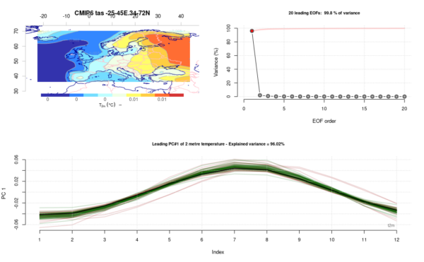
Fig 1. Leading common EOF for the mean seasonal cycle in surface air temperature (TAS) over the Euro-CORDEX region, with the spatial covariance structure in the upper left panel, variance explained (based on eigenvalues) upper right, and principal components in lower panel. Black curve represents the ERA5 reanalysis, the red curve represents CMIP5 RCP4.5 simulations and green curves CMIP6 SSP245 (see Benestad et al. (2023) for more details).
Fig 1. suggests that the GCMs do in general reproduce the mean annual cycle over Europe quite well.
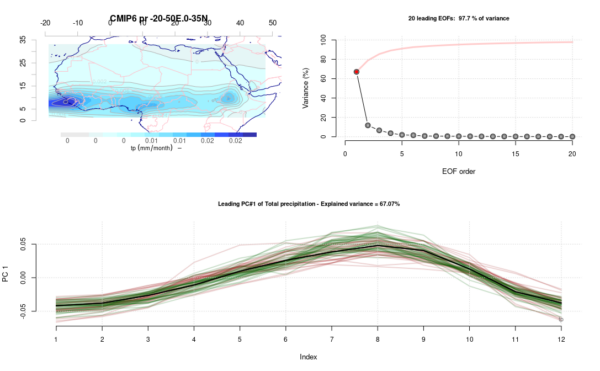
Fig. 2. Similar as Fig. 1, but for precipitation over parts of Africa.
The GCMs reproduce the seasonal variations in rainfall north of the equator near western Africa, and the leading mode accounts for 67% of the variance (Fig. 2). There is some “slack” in terms of some variations in the rainfall patterns, seen through medium-high variance estimates and scatter around the black curve in the lower panel.
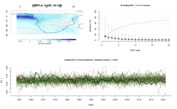
Fig. 3. Common EOFs estimated for annual precipitation over southern Africa.
Fig.3 shows an evaluation of the interannual variability in the annual rainfall, and the lower variance associated with the leading mode (13%) and the large scatter around the black curve in the lower panel suggests that the GCMs simulate a large variation of annual rainfall amounts. Nevertheless, the GCMs (red and green curves) tend to embed the ERA5 (black), suggesting that they nevertheless do reproduce the statistics somewhat reasonably.

Fig. 4. Common EOFs estimated for the mean seasonal cycle in the mean sea-level pressure (PSL) over the Indian subcontinent. Otherwise similar to Fig. 1.
It’s interesting to see if the GCMs can reproduce the mean seasonal variations in the mean sea-level pressure over southeast Asia, as it has great implications for the Indian monsoon. Fig. 4. suggest that the CMIP6 (green curves) cluster more tightly around ERA5 than the CMIP5 (red) for the leading mode that accounts for 94% of the variance.
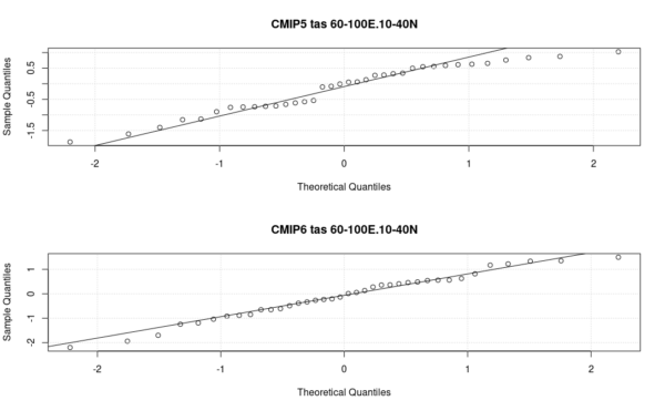
Fig. 5. Quantile-quantile plots of the principal components of the CMIP5 and 6 ensemble for a single year gives an indication as to whether the ensemble is close to being normally distributed. Here CMIP6 has results which are closer to normally distribution than CMIP5.
Fig. 5 suggests that the ensembles for the selected year approximately follow a normal distribution. This may suggest that we can summarise salient information about the ensemble with a the mean and standard deviation and hence can give an approximate description of regional natural variability similar to that Deser et al. (2012) describe.
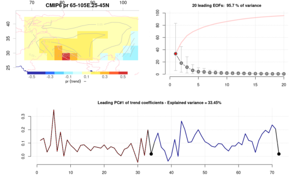
Fig. 6. Common EOFs applied to trend maps over the Tibetan Plateau, where each data point in the lower panel represents one model. Red for CMIP5 and blue for CMIP5 – ERA5 trends are repeated twice as big black circular symbols.
When we evaluate past trend patterns, we see from the modest fraction of the variance that is accounted for by the leading modes in Fig. 6 that the GCMs indicate a variety in the geographical distribution of annual precipitation changes over the Tibetan Plateau.
The climate models reproduce the regional variations quite well
These figures are in line with those for the Nordic region presented by Benestad et al. (2023). All (black, red and green) curves in the lower panels of Fig. 1-4 represent weights for the exactly same spatial covariance pattern (shown in respective upper left panels), and hence are directly comparable. Furthermore, the leading modes in Fig. 1 & 4 account for almost all of the variance in the data, leaving little room to other types of variability. The black curves are embedded inside the scatter of red and green lines, indicating that the GCMs do reproduce the salient regional climatic variation found in ERA5.
When it comes to the annual mean precipitation trends over the Tibetan Plateau, there is less of a close match between GCMs and ERA5. The relatively low fraction (33%) that the leading mode represents suggests that different GCMs tend to reproduce different trend patterns. Furthermore, the ERA5 is associated with weights that are in the lower range of the GCMs (lower panel, Fig. 6).
If you are interested in trying out common EOFs, there are some YouTube videos that provide tips: A brief presentation of common EOFs in R-studio and common EOFs for evaluation of geophysical data and global climate models. The material for the figures presented here (PDF with results for the extended analysis of Benestad et al. (2023) for the Arctic, Euro-CORDEX, Africa and Asia) is available from FigShare.
References
C. Deser, R. Knutti, S. Solomon, and A.S. Phillips, “Communication of the role of natural variability in future North American climate”, Nature Climate Change, vol. 2, pp. 775-779, 2012. http://dx.doi.org/10.1038/nclimate1562
R.E. Benestad, A. Mezghani, J. Lutz, A. Dobler, K.M. Parding, and O.A. Landgren, “Various ways of using empirical orthogonal functions for climate model evaluation”, Geoscientific Model Development, vol. 16, pp. 2899-2913, 2023. http://dx.doi.org/10.5194/gmd-16-2899-2023